How Elixir Lays Out Your Data in Memory

Higher-level languages hide the details to boost developer experience and productivity. However, this leads to a loss of understanding of the underlying system, preventing us from squeezing the highest level of efficiency and performance from our programs. Memory management is one of the aspects abstracted away from us in this trade-off. In this series, we'll take a look at how the BEAM VM works in this regard and learn to make better decisions when writing Elixir code.

What is memory management

Programs operate on top of values or a collection of values. These values are stored in memory so that they may be referred back to whenever needed to perform a particular operation. Understanding the underlying memory representation grants us the ability to adequately choose which data structures to use in a particular use-case.

Doing it by hand

Talking about memory management usually throws some programmers back to when they first learned C. This low-level language offers some functions, such as malloc and free, which, in turn, empower developers to seize and liberate memory at will:

int *my_array;
my_array = (int *) malloc(sizeof(int) * 5);
free(my_array);

However, eagle-eyed programmers (or those who have fallen into that trap before) may ask what happens if we don't call free when we no longer need the array? It leads us to a problem commonly known as a memory leak.

Memory is like a jar of nails. When our program first starts, this jar is full and may be used at will. However, not putting the nails back into the jar when we no longer need them can eventually lead to not having enough nails to do our job. The memory in our system is our jar, and we ought to keep track of our nails or risk running out of them. This is the premise for a low-level language with manual memory management, such as C.

Letting go of the training wheels

For contrast, we can look at higher-level languages, such as Elixir, which take care of this matter for us:

input = [1, 2, 3, 4, 5]
my_list = Enum.map(input, fn(x) -> x * 2 end)

In the above example, we are able to map some input of unknown length into a list without having to allocate memory for my_list in any way whatsoever. In truth, it's difficult to give a direct counter-example to the C code shown previously since there really is no way of dealing with memory in Elixir. But, if we can't free these variables from memory, doesn't it mean we'll cause a leak? Fortunately, this kind of language also takes care of this for us via a mechanism called garbage collection.

Garbage collection in the BEAM world warrants an article on its own. , to keep it short, the VM knows to keep track of which variables will be used in the future and which ones can be deleted from memory. There are many different implementations for garbage collection across a variety of languages, each with its own benefits and drawbacks.

Knowledge is power

Even though Elixir handles memory allocation for us, it still has to be done, somehow, under the hood. Thus, understanding how this is performed and how BEAM data types are operated (e.g., created, read, and modified) and represented in memory can lead us to different choices in our programs.

Our system's memory footprint and performance are affected by these decisions. Furthermore, having insight into the relationship between software and hardware rewards developers with better reasoning skills. These may come in handy when debugging weird errors or implementing mission-critical features.

Information about Elixir's BEAM VM is scarce and can be convoluted and difficult to understand. Therefore, this article aims to present developers the fundamentals of memory management and aggregate all the scattered knowledge about this topic in one place.

Memory word is the word

A word is the fundamental data unit for a given computer architecture; thus, it varies from 4 bytes to 8 bytes for 32-bit and 64-bit systems, respectively. To discover the word size of a running system, you can use the :erlang.system_info(:wordsize) function.

iex(1)> :erlang.system_info(:wordsize)
8

All data structures in Erlang are measured in this unit, and you can find the size of words using the :erts_debug.size/1 and :erts_debug.flat_size/1 functions. However, keep in mind that these are undocumented APIs and are not suited for production usage.

Bite-sized bytes: literals and immediates

The most basic memory containers in the BEAM world are immediates. These are types that fit into a single machine word. Immediates may be small integers large integers use bignum arithmetic for representation, local process identifiers (PIDs), ports, atoms, or a NIL value (which stands for the empty list and should not be confused with the atom nil).

Atoms

Atoms are the most distinct of the immediates. They fill a special atom table and are never garbage-collected. This means once an atom is created, it will live in memory until the system exits. The first 6 bits of an atom are used to identify the value as an atom type. The remaining 26 bits represent the value itself. Thus, we are left with \(2^6 = 32M\) available slots in the atom table (for both 32-bit and 64-bit systems).

When a given atom is created more than once, its memory footprint does not double. Instead of copying atoms, references are used to access the respective slot in the table. This can be seen when using the :erts_debug.size/1 function with an atom argument:

iex(1)> :erts_debug.size(:my_atom)
0

The word size is zero because the atom itself lives in the atom table, and we are just passing references to that particular slot.

A famous gotcha in the Erlang world is that exhausting the atom table crashes BEAM. Although the table has up to 32M slots, as we saw, it can be vulnerable to external attacks. Parsing external input to atoms can cause a long-running VM to crash. Therefore, it's considered a best practice to parse external input to strings whenever appropriate (for example, an HTTP endpoint's parameters).

Boxed values

Not all values fit into a single machine word. BEAM VM uses the concept of boxed values to accommodate larger values. These are made of a pointer that refers to three parcels:

1. Header: 1 word to detail the type of boxed value.
2. Arity: 26 bits, indicating the size of the following Erlang term.
3. An array of words: the length is equal to the arity defined in the previous parcel. These words contain data for the data structure at hand.

Boxed values encompass the data types not covered by immediates: lists, tuples, maps, binaries, remote PIDs and ports, floats, large integers, functions, and exports. In this article, we'll focus on the first four types.

Lists

In a BEAM VM, lists are implemented as single-linked lists and are comprised of cells. Each cell is split into two parts:

1. The value of the particular list element. For example, the value of the first element of [1, 2, 3] is 1.
2. The tail, which points to the next element in the list. Each tail keeps pointing to the next element until the last tail points to the NIL value, which represents an empty list.

In a sense, an Erlang list can be seen as a pair where the first part is the value of the list element, and the second part is another list. The next picture illustrates this concept for the list [1, 2, 3]:

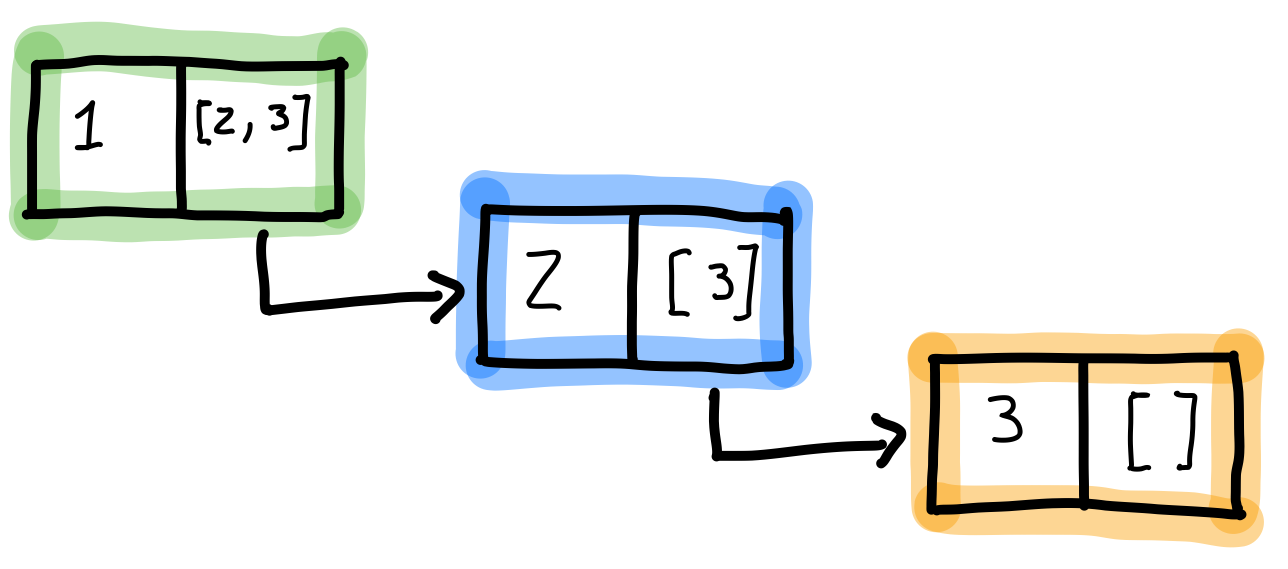
This choice of implementation is not without its benefits and trade-offs. Since it is a single-linked list, it can only be traversed forward. This is cumbersome when finding the length of a list because all the elements must be traversed. Thus, this operation is O(n) in Big-O Notation.

However, this is advantageous when adding a new element to the head of a list - achieved by this syntax [1 | [2, 3, 4]][^This is called consing, or the cons operator in the functional programming world]. Since the tail points to the remainder of a list, as in the previous example, the VM just needs to create a new cell with the value of 1 and a tail pointing to the existing list, [2, 3, 4].

Only a new head must be created in memory, and the rest of the list can be reused. This leaves us with O(1) constant time. In contrast, appending lists ([1, 2, 3] ++ [4, 5, 6]) is O(N), with N being the length of the first list. The VM must traverse its N elements to find the last one and point it to the second list instead of the NIL value.

Similarly, the reverse operation (e.g., :lists.reverse/1 or Enum.reverse/1) is also O(N). Again, BEAM just traverses the original list and copies each element to the head of the new list. Other operations, such as calculating the intersection between two lists ([1, 2, 3] -- [4, 5, 6]), incur harsher penalties when it comes to time complexity. In this operation, for each element on the first list, the second one must be traversed to check whether it exists and add it to a new list if this is the case. Therefore, we must consider a O(N) * O(M) complexity. In situations where the intersection of two lists must be calculated, employing another data structure, such as a Set, can result in better performance or memory efficiency.

The last aspect to consider in lists is locality of reference in memory, especially spatially. In short, it's how close together each element of a list is in memory. When it comes to lists, their elements have a high likelihood of being contiguous when the list was built in a loop. This is beneficial and desirable since, most of the time, elements are to be accessed in succession.

Tuples: fast access, slow modification

Next in our discussion of the topic of boxed values is the concept of tuples, which is a type of data structure that allows a defined number of elements to be grouped together. However, unlike lists, tuples are implemented using an array underneath. The following picture illustrates how the tuple {"May", 42, :ok} is prefixed by its arity, followed by the array of elements.

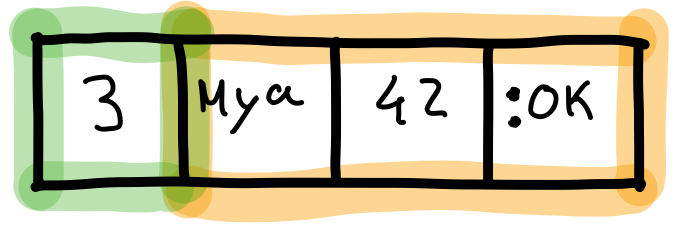
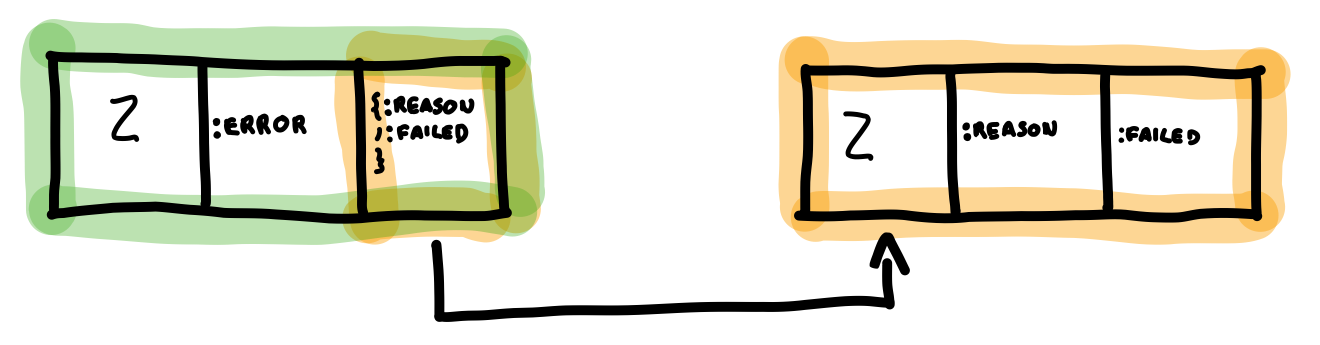
The memory used by a tuple can also be understood from the picture. The arity is stored in a single word, and each element of the array also occupies one word. Therefore, a tuple uses \(1 + arity\) words of memory. When it comes to nested tuples, this formula has to be applied to each one and summed. This is showcased in the next example, where the tuple {:error, {:reason, :failed}} has a nested tuple, which is just referred by a pointer in the parent tuple.

iex(1)> child = {:reason, :failed}
{:reason, :failed_to_start}
iex(2)> parent = {:error, child}
{:error, {:reason, :failed}}
iex(3)> :erts_debug.size(parent)
6

Both the parent and child tuple have arity 2 (or 3 memory words each). After summing both, we get a total of 6 words, as returned by the :erts_debug.size/1 function. Choosing to use arrays grants tuples O(1) constant access time for both building and n-th element lookup.

Nonetheless, modifying[^The word modifying, in this context, is used to imply creating the same tuple but with a different element at a given position. True modification is impossible since everything in a BEAM VM is immutable.] an element in a tuple is O(N). Like everything in the Erlang world, the arrays used by tuples are immutable. The implications of such an implementation are that the tuple must be traversed and each element copied (except the altered element, which will be different).

Memory locality for tuples can be trickier when compared to lists. Although the use of arrays grants contiguous memory blocks for tuple elements, they can become scattered when nested tuples (like the one depicted above) are not created simultaneously.

Between tuples and lists are maps

Maps provide a good middle-ground choice for those who are concerned about both lookup and update performance. Their implementation diverges based on the size of the map itself. Maps up to 31 keys rely on a sorted key-value list, and maps larger than that can be changed to use a hash-array mapped trie, a kind of associative array. This achieves O(log n) for insert and lookup operations, although two implementations are at hand.

In a "small map" implementation, inserting and looking up involves applying a searching algorithm to find the correct position inside the sorted list. On a list of up to 31 elements, this takes 5 iterations at most with an algorithm like binary search. When it comes to "large maps", the data structure in place also provides the same time complexity for these operations. Keep this in mind when using maps in your programs, as one may be prone to believe this data structure yields O(1) time complexity for the mentioned operations, similar to hash maps provided by other languages.

For most use-cases, the use of maps or tuples can be considered interchangeable. For example, rarely are more than 10 fields used when storing the state of a process (like a GenServer). This means that either a tuple or a map can be used without any noticeable performance penalty. This is detailed by Steve Vinoski is a well-known Erlang expert and a co-author of the Designing for Scalability with Erlang/OTP book] in this post.

Nonetheless, in performance-critical code, operations like element lookup (which, as we saw, are O(1) in tuples and O(log n) in maps) can make a difference, and it's up to the developer to choose the right data structure based on the system's needs. On such occasions, Erlang's records can come in quite handy, as they offer accessor functions similar to Elixir's struct but better performance in tight loops, as explained by José Valim himself.

Binaries: to share or not to share

Binary sequences are different since they may be shared between processes or be local to a given process. We can distinguish binaries as follows in the next few sections Erlang's Binary Handling Guide can be a good supplemental reference for this topic (note that some of these intricacies can best be observed in code by passing the ERL_COMPILER_OPTIONS=bin_opt_info environment variable when compiling).

Heap binaries

Usually abbreviated as HeapBin, the size of these binaries is under 64 bytes. They are stored in the local process' heap and are not shared with other processes. Thus, when they are sent in a message, the entire binary is copied to the receiving process. When a binary becomes stale, it's cleaned up by the process' garbage collection.

Reference-counted binaries

Reference-counted binaries are usually abbreviated as RefcBin. The size of these binaries is equal or larger than 64 bytes. They are stored in a dedicated and shared binary heap. Whenever a process uses a RefcBin, a corresponding process binary (or ProcBin) is created in its heap. A ProcBin acts as a reference to the RefcBin. The binary heap keeps the total reference count for each of its binaries separately. The count for a given binary is incremented when a new reference is created or decremented once a reference becomes stale.

This reference-counting mechanism offers the advantage of processes just passing the reference to each other instead of copying the entire binary when exchanging messages. However, these binaries are more prone to memory leaks, and garbage collection of these shared binaries is dependent on the liveness of their respective references.

Only after all the references have become stale and cleaned up - by their own process's garbage collection - will the RefcBin be cleaned up. However, if just one of the processes holds on to the reference, the large binary will keep on living in memory. This may eventually lead to a binary leak

As you may be aware, all data in BEAM are immutable. This prevents a large class of bugs around shared memory. As processes cannot access or modify each other's memory areas, problems like race conditions are eliminated. Nonetheless, this comes at the expense of having processes always copying data to each other - when communicating - instead of sharing.

Since a BEAM VM is aimed at building low-latency and high-throughput I/O systems, which have to handle binaries with ease, the choice of sharing binaries larger than 64 bytes may have been a workaround to keep performance and efficiency up to par. Like always, engineering is a game of trade-offs.

Sub binaries

A sub binary object is a reference to a slice of either a HeapBin* or a _RefcBin*. These are created when matching a part of one of these binaries and exist in the process' heap.

Match contexts

Similar to the sub binary, match contexts are a reference optimized for matching slices of binaries. Match contexts are a compiler optimization and only happen when it knows a sub-binary will be discarded soon after its creation. This is best exemplified in Erlang's Binary Handling Guide. Like sub-binaries, these also live in the local process' memory area.

Conclusion

In this article, we explained how each data type inside BEAM is allocated in memory. We also saw how the underlying implementation of these data structures can affect the common operations we rely on and how they may affect our programs.

Keeping this information in mind (or in the form of a cheat-sheet) can boost our programs' performance or reduce their memory footprints. At the very least, we end up with a better understanding of how things work under the hood.